Visualizing Results
While not limited to any domain in particular, attribution methods are most
commonly applied on 2-dimensional image data. For this reason, Zennit implements
a few functions to aid in the visualization of attributions of image data as
heatmaps. These methods may be found in zennit.image. To simply save
tensors that can be represented as images (1 or 3 channels, 2 dimensions), with
or without heatmap, zennit.image.imsave() may be used.
Let us consider the following setting which simulates image data:
import torch
from torch.nn import Sequential, Conv2d, ReLU, Linear, Flatten
from zennit.attribution import Gradient

# setup the model
model = Sequential(
    Conv2d(3, 8, 3, padding=1),
    ReLU(),
    Conv2d(8, 16, 3, padding=1),
    ReLU(),
    Flatten(),
    Linear(16 * 32 * 32, 1024),
    ReLU(),
    Linear(1024, 10),
)
# some random input data
input = torch.randn(8, 3, 32, 32, requires_grad=True)

# compute the gradient and output using the Gradient attributor
with Gradient(model) as attributor:
    output, relevance = attributor(input)
The relevance has the same shape as the input, which here is (8, 3, 32, 32).
We can save the output and relevance, with all color-information intact, by
simply doing:
from zennit.image import imsave

for n, (inp, rel) in enumerate(zip(input, relevance)):
    imsave(f'input_{n:03d}.png', inp.detach())
    imsave(f'relevance_{n:03d}.png', rel)
Alternatively, the images may be composed as a grid, and saved as a single image:
imsave('input_grid.png', input.detach(), grid=True)
imsave('relevance_grid.png', relevance, grid=(2, 4))
The keyword argument grid may either be boolean, or the 2d shape of the image grid.
While this works well for the input, it is hard to interpret the attribution from the resulting images. Be aware that commonly input images are pre-processed before they are fed into networks. While clipping and scaling the image pose no problem for its visibility, normalization will change the look of the image greatly. Therefore, when saving images during training or inference, it is recommended to visualize input images either before applying the normalization, or after applying the inverse of the normalization.
imsave() uses zennit.image.imgify(), which,
given a numpy.ndarray or a torch.Tensor, will return a
Pillow image, which can also be used to quickly look at the image without saving
it:
from zennit.image import imgify

image = imgify(input.detach(), grid=True)
image.show()
Heatmap Normalization
Commonly, a heatmap of the attribution is produced by removing the color-channel
either by taking the (absolute) sum and normalizing to fit into an interval.
imsave() (through imgify()) will
shift and scale the input such that the full range of colors is used, using the
input’s minimum and maximum respectively. This can be tweaked by supplying the
vmin and vmax keyword arguments:
absrel = relevance.abs().sum(1)
# vmin and vmax works for both imsave and imgify
imsave('relevance_abs_0.png', absrel[0], vmin=0, vmax=absrel[0].amax())

image = imgify(absrel[0], vmin=0, vmax=absrel[0].amax())
image.show()
Another way to normalize the attribution which can be used with both
imsave() and imgify() is to use
the symmetric keyword argument, which provides two normalization strategies:
symmetric=False (default) and symmetric=True. Keep in mind that the
normalization of the attribution can greatly change how interpretable the
heatmap will be.
Let us consider a more interesting image to compare the two normalization strategies with signed and unsigned data:
from itertools import product

grid = torch.stack(torch.meshgrid(*((torch.linspace(-1, 1, 128),) * 2), indexing='xy'))
dist = ((grid + 0.25) ** 2).sum(0, keepdims=True) ** .5
ripples = (dist * 5 * torch.pi).cos().clip(-.5, 1.) * (-dist).exp()

for norm, sign in product(('symmetric', 'unaligned'), ('signed', 'absolute')):
    array = ripples.abs() if sign == 'absolute' else ripples
    symmetric = norm == 'symmetric'
    imsave(f'ripples_{norm}_{sign}_bwr.png', array, symmetric=symmetric)
    imsave(f'ripples_{norm}_{sign}_wred.png', array, symmetric=symmetric, cmap='wred')
The keyword argument cmap is used to control the color map.
|
|
|
|
|
|---|---|---|---|---|
signed |
absolute |
signed |
absolute |
|
|
|
|
|
|
|
|
|
|
|
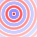
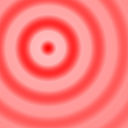

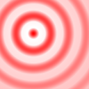
Negative values were clipped to better see how the normalization modes work.
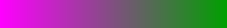
The default color map is 'bwr', which maps 0.0 to blue, 0.5 to white and 1.0 to
red, which means it is a signed color map, as the center of 0.5 is a
neutral point, with color intensities rising for values below and above.
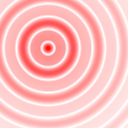
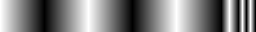
Color map 'wred' maps 0.0 to white and 1.0 to red, which makes it
an unsigned color map, as its color intensity is monotonically increasing.
Using symmetric=False will simply map [min, max] to [0., 1.], i.e the
minimum value to 0.0, and the maximum value to 1.0. This works best with
unsigned color maps, when relevance is assumed to be monotonically increasing
and a value of 0.0 does not have any special meaning.
symmetric=True will find the absolute maximum per image, and will map the
input range [-absmax, absmax] to [0., 1.]. This means that the result
will be centered around 0.5, which works best with signed color maps (like
'bwr'), as positive (here red) and negative (here blue) intensities in the
produced heatmap are made comparable.
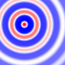
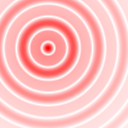
In the example above, our input is in the range [-0.5, 1.0]. If the negative
and positive values are meaningful (generally the case for attribution methods),
and the color map has a meaningful value at 0.5 (i.e. is signed),
symmetric=True is usually the best choice for normalization.
For symmetric=False the example above shows that with 'bwr' gives the
illusion of a shifted center, which makes it look like the attribution is
predominantly negative. Using the monotonic wred is normally the better
choice for the symmetric=False, but with signed attributions
the results are not as clear as they can be.
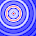
Finally, the example above shows the different outcomes when the input is
signed or its absolute is taken.
Using vmin and vmax overrides the minimum and maximum values
respectively determined by the normalization mode.
This means that, for example, using vmin=0 (and not setting vmax) with
symmetric=True will clip all values below 0.
Another useful setting is when the input is positive (or its absolute value was
taken) to use vmin=0 with symmetric=False, as this will give the full
range from 0 to the maximum value, since the smallest value may be larger than 0
when in cases where it is known that 0 would be the smallest possible value.
This shows the importance of the choice of the normalization and the color map.
Color Maps
Color maps play an essential role in the production of heatmaps which highlight
points of interest best. With the normalization modes we have seen the built-in
signed color map bwr (blue-white-red) and unsigned color map wred
(white-red).
All built-in color maps are defined in zennit.image.CMAPS.
The built-in unsigned color maps are:
Identifier |
CMSL-Source |
Visualization |
|---|---|---|
|
|
|
|
|
|
|
|
|
|
|
|
|
|
|


and the built-in signed color maps are:
Identifier |
CMSL-Source |
Visualization |
|---|---|---|
|
|
|
|
|
|
|
|
|
|
|
|
|
|
|
|
|
|


CMSL-Source is the source code of the color map in Color-Map Specification
Language (CMSL). The color map for imsave() and
imgify() may be specified in one of three ways: the
identifier of a built-in color map (wred, coldnhot, …), a string
containing CMSL source-code, or a zennit.cmap.ColorMap instance.
from zennit.cmap import ColorMap

bar = torch.arange(256)[None].repeat((32, 1))
imsave('bar_wred.png', bar, cmap='wred')
imsave('bar_string.png', bar, cmap='ff0,00f')
cmap = ColorMap('000,f00,fff')
imsave('bar_cmap.png', bar, cmap=cmap)
Color-Map Specification Language
Color-Map Specification Language (CMSL) is a domain-specific language to
describe color maps in a quick and compact manner. It is implemented in
zennit.cmap. Color-maps can be compiled using the
zennit.cmap.ColorMap class, of which the constructor expects
CMSL source code as a string. Alternatively, a ColorMap instance may be obtained
using zennit.image.get_cmap(), which first looks up its argument string
in the built-in color-map dictionary zennit.image.CMAPS, and, if it
fails, tries to compile the string as CMSL source code.
from zennit.cmap import ColorMap
from zennit.image import get_cmap

bar = torch.arange(256)[None].repeat((32, 1))

cmap1 = ColorMap('000,a0:f00,fff')
cmap2 = get_cmap('1f:fff,f0f,000')

img1 = imgify(bar, cmap=cmap1)
img2 = imgify(bar, cmap=cmap2)

img1.show()
img2.show()
CMSL follows a simple grammar:
cmsl_cmap  ::= color_node ("," color_node)+
color_node ::= [index ":"] rgb_color
index      ::= half | full
rgb_color  ::= half half half | full full full
full       ::= half half
half       ::= <single hex digit 0-9a-fA-F>
Values for both index and rgb_color are specified as hexadecimal values
with either one (half) or two (full) digits, where index consists of
a single value 0-255 (or half 0-15) and rgb_color consists of 3 values 0-255
(or half 0-15).
The index of all color_nodes must be in ascending order.
It describes the color-index of the color-map, where 00 (or half 0) is
the lowest value and ff (i.e. decimal 255, or half f) is the highest
value.
The same value of index may be repeated to produce hard color-transitions,
however, using the same value of index more than twice will only use the two
outermost color values.
If the indices of the first or last color_nodes are omitted, they will be
assumed as 00 and ff respectively.
Two additional color_nodes with the same color as the ones with lowest and
highest index will be implicitly created at indices 00 and ff
respectively, which means that if the lowest and/or highest specified color node
indices are larger or smaller than 00 or ff respectively, the colors
between 00 and the lowest index, and the highest index and ff will be
constant.
A color map needs at least two color_nodes (i.e., a useless single-color
color-map cannot be created by specifying a single color_node).
A color node will produce a color of its rgb_color for the value of its index.
Colors for values between two color nodes will be linearly interpolated between
their two colors, weighted by their respective proximity. Color nodes without
indices will evenly spaced between color nodes with indices. The first and last
color nodes, if not equipped with an index, will be assumed as 00 and ff
respectively.
While technically there does not exist a syntactic difference between signed
and unsigned color maps, signed color maps often require a color node at the
central index 80, while unsigned color maps should have monotonically
increasing or decreasing intensities, which can be most easily done by only
specifying two color nodes.
The built-in color map cold could be understood as a signed color map,
since it has an explicit color node blue at its center. Visually, however,
due to its monotonicity, it is hard to interpret as such.
The following shows a few examples of color maps along their CMSL source code:
CMSL-Source |
Visualization |
|---|---|
|
|
|
|
|
|
|
|
|
|
|
|


Additionally, zennit.cmap.LazyColorMapCache may be used to define
color maps in bulk, and lazily compile them when they are accessed the first
time. This is the way the built-in color maps are defined in
zennit.image.CMAPS.
from zennit.cmap import LazyColorMapCache
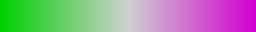
cmaps = LazyColorMapCache({
'reds': '111,f11',
'blues': '111,11f',
'greens': '111,1f1',
})
img = imgify(ripples, cmap=cmaps['greens'])
img.show()
LazyColorMapCache stores the specified source code for
each key, and if accessed with cmaps[key], it will either compile the
ColorMap, cache it if it has not been accessed
before and return it, or it will return the previously cached
ColorMap.
Changing Palettes
When using imgify() (or
imsave()), arrays with a single channel are converted
to PIL images in palette mode (P), where the palette specifies the color
map. This means that the color map of an image may be changed later without
modifying its values. The palette for a color map can be generated using its
zennit.cmap.ColorMap.palette() method.
palette() accepts an optional argument level
(default 1.0), with which the resulting palette can be either stretched or
compressed, resulting in heatmaps where either the maximum value threshold is
moved closer to the center (level > 1.0) or farther away from it (0.0 < level
< 1.0). A value of level=2.0 proved to better highlight high values of
a heatmap in print.
img = imgify(ripples, symmetric=True)
img.show()

cmap = ColorMap('111,1f1')
pal = cmap.palette(level=1.0)
img.putpalette(pal)
img.show()
The convenience function zennit.image.palette() may also be used to
directly get the palette from a built-in color map name or CMSL source code.
This way, existing PNG-files of heatmaps may thus also be modified to use different color maps by changing their palette:
from PIL import Image
from zennit.image import palette

# store a heatmap
fname = 'newheatmap.png'
imsave(fname, ripples, symmetric=True)

# load the heatmap, change the palette and write it to the same file
img = Image.open(fname)
img = img.convert('P')
pal = palette('f1f,111,ff1', level=1.0)
img.putpalette(pal)
img.save(fname)
A utility CLI script which changes the color map is provided in share/scripts/palette_swap.py, which can be used in the following way:
$ python share/scripts/palette_swap.py newheatmap \
     --cmap 'f1f,111,ff1' \
     --level 1.0